| Scenario | True ORR (B1 < 50) |
True ORR (B1 ≥ 50) |
P(Enrich) | Median B1 Cutoff |
N Enriched |
Go Rate (overall) [1] |
Go Rate (enriched) [2] |
Go Rate (not enriched) [3] |
E[ORR] Final Pop |
|---|---|---|---|---|---|---|---|---|---|
| Null - Inactive (flat ORR = 0.15) | 15.0% | 15.0% | 20.3% | 85.0 | 216 | 0.0% | 0.0% | 0.0% | 15.1% |
| Null - Boundary (flat ORR = 0.25) | 25.0% | 25.0% | 50.6% | 65.0 | 175 | 34.7% | 48.6% | 20.4% | 26.0% |
| Null - Inverted B1 effect (high ORR in low B1) | 25.0% | 10.0% | 1.4% | 80.0 | 216 | 0.0% | 0.0% | 0.0% | 17.4% |
| Active - Global effect (flat ORR = 0.35) | 35.0% | 35.0% | 18.8% | 15.0 | 256 | 100.0% | 100.0% | 100.0% | 35.3% |
| Active - Strong B1 effect (step at 50) | 10.0% | 35.0% | 99.9% | 65.0 | 201 | 99.6% | 99.7% | 0.0% | 35.4% |
| Active - Moderate B1 effect (step at 50) | 15.0% | 30.0% | 95.9% | 75.0 | 162 | 86.5% | 90.2% | 0.0% | 30.3% |
| Active - Weak B1 effect (shallow gradient) | 15.8% | 25.4% | 90.9% | 85.0 | 147 | 71.7% | 78.9% | 0.0% | 28.9% |
Adaptive Enrichment
Trial Design
Biomarkers
Bayesian
A practical explainer of adaptive enrichment in biomarker-driven oncology, illustrated with a single-arm Bayesian phase 2 example.
In early-phase oncology, selecting the appropriate patient population is key to demonstrating efficacy of a therapy. This is especially true for drugs with a mechanism of action linked to a biomarker: if the target population is mis-specified, the efficacy signal can be diluted or missed altogether.
Adaptive enrichment allows for changing the biomarker threshold for enrolment during your study, in order to better target patients who are expected to respond. This means you don’t have to commit to a biomarker cut-off at the start of your study (based on potentially limited Phase 1 data), and can mean the final trial population will contain a higher proportion of responders.
This article will outline operational and statistical mechanisms for adaptive enrichment, through a worked example of a Phase 2 single-arm trial.
NotePerspective
Project Optimus has put a spotlight on trial design for early-phase oncology, and more recently, FDA have highlighted Bayesian methods via issuing a draft guidance. The natural next step in biomarker-driven oncology is a focus on advanced and innovative designs to enhance patient selection.
Patient Selection — The “why”
The core element of adaptive enrichment is in the name — the biomarker cut-off to enrol patients and the corresponding inclusion/exclusion criteria can be adaptively changed throughout the trial.
This allows you to enrol a higher proportion of patients who are expected to respond, and gives flexibility that the biomarker cut-off does not need to be fixed at the beginning of the trial. This is particularly useful when running a larger Ph2 trial — you may only have limited Ph1 or Ph2a data regarding the biomarker–response relationship. By using adaptive enrichment, you can re-assess this relationship and the corresponding cut-off part-way through your trial. The end result being that you will enrol more patients in the “active region”, and gain a greater understanding of the biomarker–response mechanics and efficacy of your drug.
Adaptive Enrichment — The “what”
Adaptive enrichment uses pre-specified statistical analyses to characterise the biomarker–response relationship within the patient population. Based on the outcome of pre-specified interim analyses, the biomarker threshold can be updated.
Similar to a cohort review during dose escalation, the statistical analysis aims to make a recommendation on whether to increase the biomarker cut-off, decrease it, or leave it unchanged.
The goal is to answer the following questions:
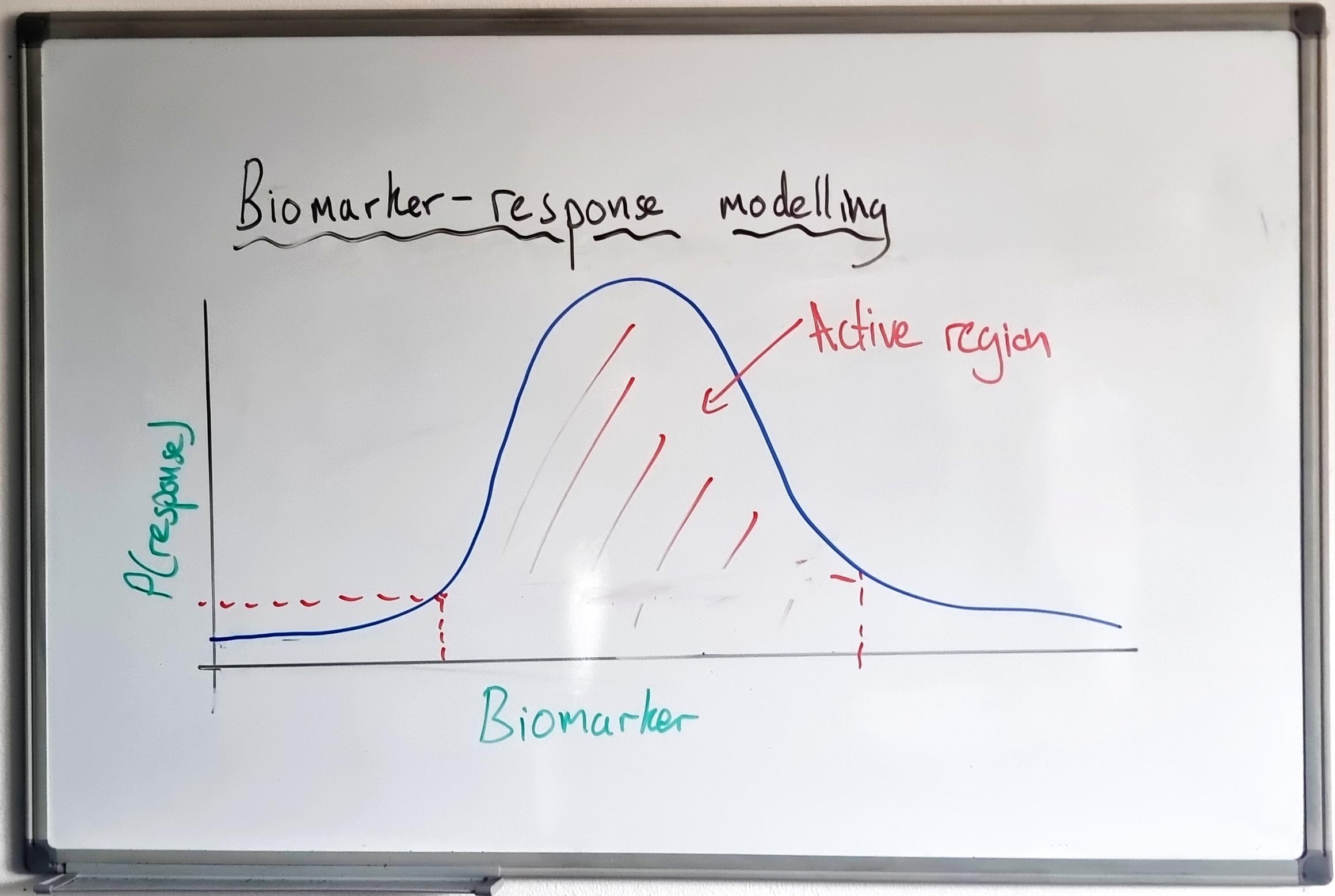
- Is there a biomarker level that corresponds to an “active region” (where clinical response is greater)?
- Does the current biomarker cut-off correspond to this “active region”?
- If not, what is an updated biomarker cut-off that would better select the active region?
Here, I modify methods proposed by Simon & Renfro1 to a single-arm Ph2 trial, drawing on Bayesian methods for continuous biomarkers developed by Tu et al.2
Trial Design
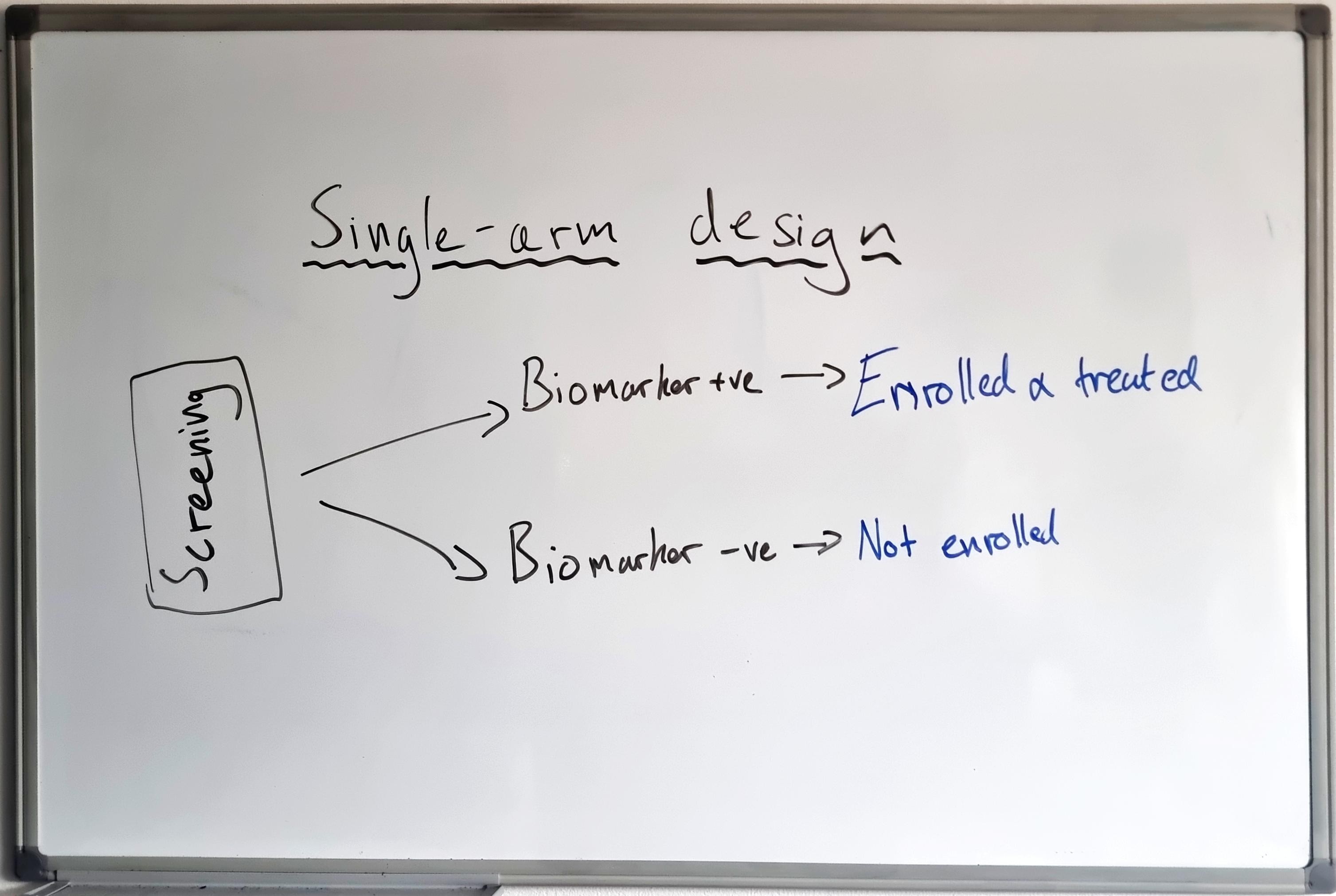
For this worked example, I am using a single-arm, Phase 2 oncology trial, which has a primary efficacy endpoint of Objective Response Rate (ORR)3 as the response variable.
In this example, the trial is initially an all-comers design — all patients are eligible regardless of their biomarker expression level — with the only requirement that biomarker expression level is collected for all patients at baseline. The total planned enrolment is n = 300, with interim analyses planned at n = 100 and n = 200. Each interim analysis models the biomarker–response relationship, with the option to adaptively modify the trial into an enrichment design by adding a biomarker cut-off to the eligibility criteria.
The goal of the interim analysis is to restrict future enrolment to only patients who have a greater chance of response (enrich). Success criteria for this is based on judge the drug to be active when we see a response of ≥ 25% ORR. The final analysis therefore consists of a Go/No-Go determination, driven by the target ORR of ≥ 25%.
As a single-arm study, this design may be particularly relevant to areas where there are limited treatment options. With no control arm there is no assessment of treatment-by-biomarker interaction, and this design on its own would not be able to determine whether the biomarker was predictive or prognostic.
Statistical Methodology
Here is how we translate this design into an operational statistical framework.
First, decide on the endpoint. Are you:
- Comparing the difference in ORR between the enriched (“biomarker positive”) vs. non-enriched (“biomarker negative”) populations, or
- Assessing the ORR in the biomarker-positive population only?
Option (1) can be a stronger statistical statement to make at the end of the trial, and option (2) can be more suited when you expect to target mostly responders (e.g. based on biomarker distribution and prevalence).
For this example, I have set the design up assuming (2) — setting the hypothesis up such that in order to deem the treatment efficacious, the enriched population must demonstrate an ORR above a certain level (“target ORR”).
Next, we want to specify our prior assumptions and the statistical mechanism by which to judge whether we should modify the design to enrich to a specified region. Bayesian methods are a natural fit for this type of design and interim decision-making. At each interim, a Bayesian Logistic Regression Model (BLRM) is fitted and the posterior probability of a specific biomarker cut-off where the ORR ≥ 0.25 is calculated, which is used to drive the enrichment decision.
For the final Go/No-Go decision, the probability of the selected region having an ORR ≥ 0.25 is used.
Mathematically:
- Interim rule: \(P(\text{ORR}(x) \geq 0.25 \mid \text{data}) > \tau\)
- Go/No-Go rule (final analysis): \(P(\overline{\text{ORR}}(B1 \geq c) \geq 0.25 \mid \text{data}) > \tau\)
Note
The posterior probability is the output from the Bayesian model — driven by the data observed so far. A higher threshold \(\tau\) at later interims reduces the risk of premature enrichment.
Bayesian methods require prior assumptions. For this example, we will use a non-informative prior — that is, we will allow the observed data to drive the biomarker–response relationship. Another option is to use data gathered from Phase 1 and Phase 2a and incorporate this into a prior to share information across trials.
Putting this all together, we end up with:
Target ORR — In this example, we are interested in a biomarker cut-off that selects a patient population with an ORR of 0.25 or greater.
Enrichment threshold — At the first interim, cast a wide net and update the cut-off based on a probability of the ORR being 0.25 or greater at 30%. For the second interim, tighten this to select the cut-off that corresponds to a 50% chance of the ORR being 0.25 or greater. For the final analysis (Go/No-Go), select a region which has an 80% probability of the ORR being 0.25 or greater. This allows us to avoid over-tightening at earlier interims where data is sparse.
Prior assumptions — Non-informative prior: observed data drives the relationship.
Final Go/No-Go — Determine if any region (all-comers or subgroup) satisfies the target ORR threshold of 0.25 or greater.
Interim Decision Making
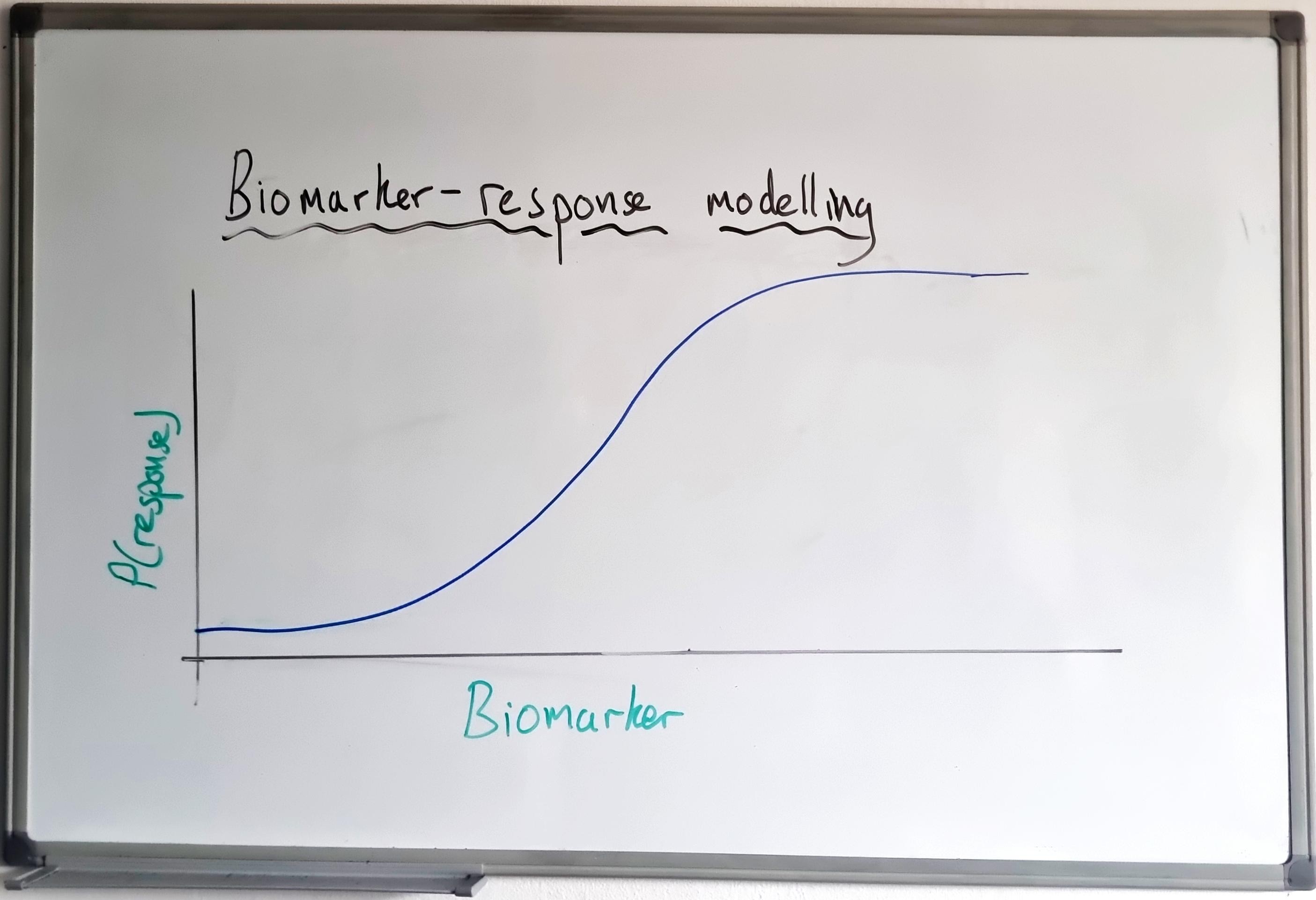
At each interim, the BLRM will be fitted for ORR ~ biomarker level, to characterise the biomarker–response relationship. A typical output is as follows: observed data (ORR by biomarker level), Model Output 1 (plot of ORR vs. biomarker level), and Model Output 2 (plot of \(P(\text{ORR} > 0.25)\) — the posterior probability plot).
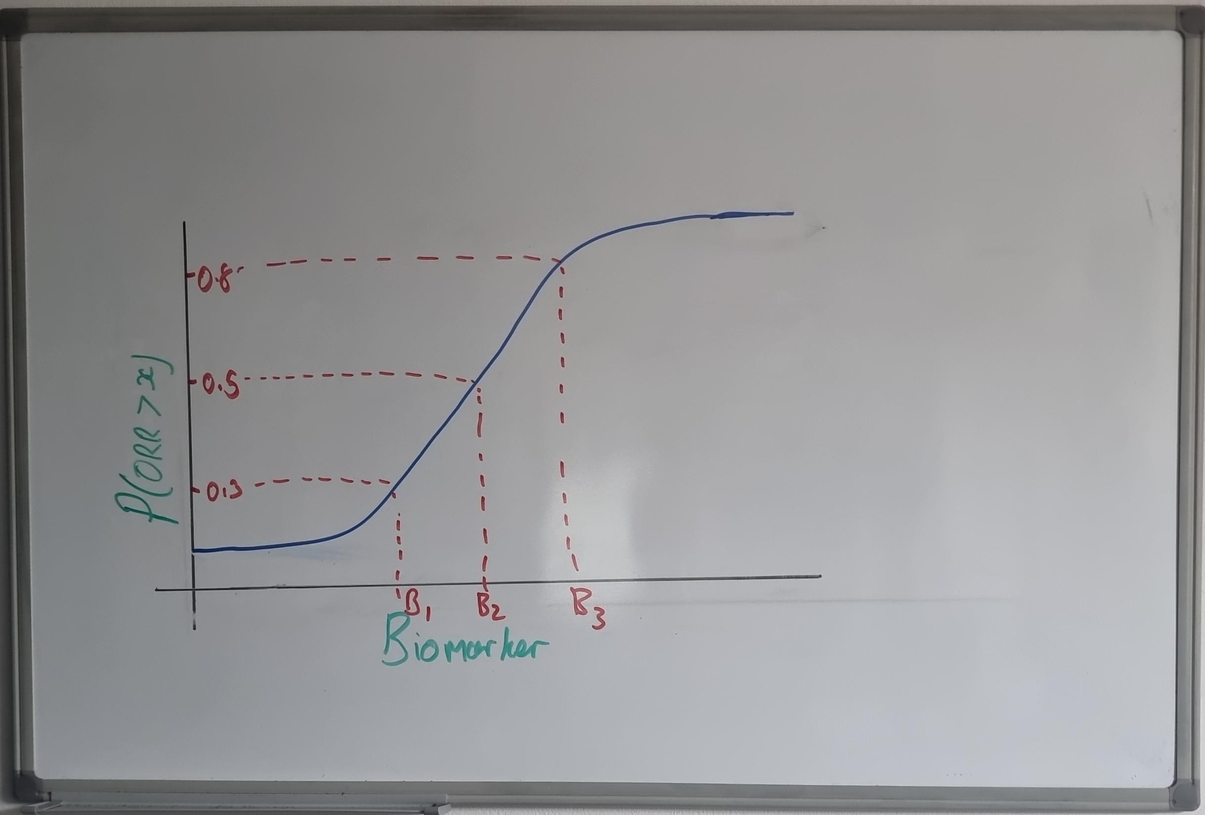
The posterior probability plot shows which biomarker values correspond to a sufficiently high probability that ORR exceeds 0.25. At each interim, these outputs are used to decide whether to enrich — is there sufficient evidence that a different biomarker cut-off will select a patient population with a higher response?
Protocol Requirements
In order to operationalise this design, the analysis methods, pre-specified interims, and decision rules must be included within your study protocol. Additionally, full simulation work must be conducted to understand the operating characteristics of the design.
To understand the operating characteristics, the full adaptive process must be simulated repeatedly under a range of plausible scenarios.
The trial is simulated to completion (interim analysis performed, enrichment decision made), and this process is repeated (for example) 1,000 times. From this, the power, Type I error, and expected biomarker cut-off are reported.
Typical scenarios cover the null scenario (to measure Type I error) along with weak to strong effect scenarios. Below are simulated operating characteristics across scenarios:
NoteAppendix: Methodology Notes
Model: Bayesian logistic regression (BLRM) with two parameters — \(\text{logit}(p_i) = \alpha + \beta \cdot B1_{i,\text{scaled}}\), where \(B1_{i,\text{scaled}} = (B1_i - 50)/50\) maps the raw biomarker to \([-1, 1]\). This assumes a monotonic (log-linear) biomarker–response relationship.
Priors: Non-informative: \(\alpha \sim N(0, 100)\), \(\beta \sim N(0, 100)\). Under this parameterisation, the prior on \(\alpha\) is effectively flat over all plausible response rates, and the prior on \(\beta\) is flat over all plausible effect magnitudes across the biomarker range.
Posterior approximation: Laplace (normal) approximation to the posterior, combining the MLE Fisher information with the prior precision. Posterior draws (\(K = 4{,}000\)) are sampled from the resulting multivariate normal.
Power = \(P(\text{conclude ORR} \geq 0.25 \text{ in the final evaluated population at Stage 3})\). For null scenarios, this is the Type I error rate.
[1] Go Rate (overall) = probability of a Go decision at Stage 3 across all simulations, regardless of whether enrichment occurred.
[2] Go Rate (enriched) = Go rate conditional on enrichment having been triggered at Stage 1 or Stage 2.
[3] Go Rate (not enriched) = Go rate conditional on no enrichment occurring (all-comers design retained).
P(Enrich) = probability that enrolment criteria are restricted to \(B1 \geq \text{cutoff}\) at any interim (Stage 1 or Stage 2).
Median B1 cutoff = median selected enrichment threshold, conditional on enrichment occurring. “—” indicates enrichment was rarely or never triggered.
N Enriched = mean number of patients enrolled after enrichment is applied (subset of \(N_{\max} = 300\)), conditional on enrichment occurring. “—” when enrichment was not triggered.
E[ORR] Final Pop = expected observed ORR in the final analysed population (all-comers if no enrichment, or \(B1 \geq \text{cutoff}\) if enriched), averaged across simulations.
Enrichment ratchet thresholds: Stage 1 = 0.30, Stage 2 = 0.50, Stage 3 (final Go/No-Go) = 0.80.
Cutoff selection strategy: At each interim, candidate cutoffs are evaluated over a grid (\(B1 \in \{20, 25, \ldots, 80\}\)). The lowest cutoff \(c\) satisfying \(P(\text{mean ORR in } B1 \geq c \geq 0.25 \mid \text{data}) \geq \text{stage threshold}\) is selected (broadest viable population).
Biomarker distribution: \(B1 \sim \text{Uniform}(0, 100)\) in the unselected population. After enrichment at cutoff \(c\), new patients are drawn from \(B1 \sim \text{Uniform}(c, 100)\).
Limitations and Extensions
Adaptive enrichment can be applied to many types of trial design and endpoints — randomised trials, trials with multiple biomarkers, time-to-event endpoints, and difference-in-response endpoints (comparative trials).
Statistically, the BLRM is a fairly rigid model that works well for simple biomarker–response relationships — for example, a “classic” monotonic relationship. Flexible models such as splines or Gaussian Processes (GP) may be more appropriate for complex biomarker–response relationships.
Summary
Adaptive enrichment utilising Bayesian modelling is a powerful approach that allows for modification of the enrolment criterion during the study - useful when the biomarker-response relationship is unknowns. Scenario simulation is a must, and is expected by reviewers. Single-arm designs have limitations.
Footnotes
Simon R, Renfro LA. Adaptive enrichment designs for clinical trials. Biostatistics 2013; 14(1): 27–35.↩︎
Tu Y, Liu Y, Mack WJ, Renfro LA. Bayesian adaptive enrichment design for continuous biomarkers. Stat Med 2025; 44(20–22): e70262.↩︎
ORR is any Complete Response (CR) or Partial Response (PR) as per RECIST 1.1.↩︎